Once data is loaded into the GIS Geographic Information Systems the software used to create, store, and manage spatial data Data that deals with location, such as lists of addresses, the footprint of a building, the boundaries of cities and counties, etc. , analyze spatial problems, and display the data in cartographic layouts Geographic Information Sciences , it is often not exactly how we need it to look, it may be outdated and in need of an update, it may be missing features, or it may have bits that are completely wrong. This is where data editing comes in.
Data editing comes in two basic types: direct feature editing The process of modifying the geometry (shape, location, or vertices) of spatial features directly on a map, such as moving a point A GIS vector data in any sort of digital science or art, is simply denoting a type of graphical representation using straight lines to construct the outlines of objects geometry type which is made up of just one vertex pl. vertices One of a set of ordered x,y coordinate pairs that defines the shape of a line or polygon feature. , marking a single XY location in any given geographic or projected coordinate system. , reshaping a polygon, or adjusting line vertices. , and attribute table editing The process of modifying the non-spatial information associated with features, such as changing field values, adding new attributes, or updating descriptive data in the table. . While both kinds are lumped together as editing, since they go hand-in-hand, to simplify the concepts behind both, we will split them up to look at why we would use one kind or the other and some basic techniques of editing in ArcMap. In the real world, however, editing refers to several tasks, such as creating new features, changing how existing features look, changing values in the attribute table, adding new values to the attribute table, and deleting features. Basically, working with GIS Geographic Information Systems the software used to create, store, and manage spatial data Data that deals with location, such as lists of addresses, the footprint of a building, the boundaries of cities and counties, etc. , analyze spatial problems, and display the data in cartographic layouts Geographic Information Sciences data is broken into four major categories: creating data, editing data, geoprocessing tools, and cartography. As we've learned so far, there are many tasks which fall into each category, but it's important to understand how these grouped tasks are referred to the in the real world.
6.4.2: Defining and Projecting Data
We spent a ton of time looking at geographic and projected coordinate systems - how the are defined, how they are created, some of the key terms which go along with them, how they display on the screen, and how we measure features (among other things). We also know that all coordinate systems, geographic or projected, are based on Cartesian coordinate systems and have two established known facts - the origin of the system and the units of the grid. Geographic coordinate systems are measured with angular units and projected coordinate systems are measured with linear units. Lastly, we understand that GIS Geographic Information Systems the software used to create, store, and manage spatial data Data that deals with location, such as lists of addresses, the footprint of a building, the boundaries of cities and counties, etc. , analyze spatial problems, and display the data in cartographic layouts Geographic Information Sciences data is stored in some coordinate system and we learned in lab how to look up which one via the properties.
A few pages back, we looked at how to create a new feature class One of the two main types of vector data in any sort of digital science or art, is simply denoting a type of graphical representation using straight lines to construct the outlines of objects we learn in this class (there are more than two vector data in any sort of digital science or art, is simply denoting a type of graphical representation using straight lines to construct the outlines of objects types in GIS). Feature classes are each only one geometry type, either a point A GIS vector data in any sort of digital science or art, is simply denoting a type of graphical representation using straight lines to construct the outlines of objects geometry type which is made up of just one vertex pl. vertices One of a set of ordered x,y coordinate pairs that defines the shape of a line or polygon feature. , marking a single XY location in any given geographic or projected coordinate system. , a polyline A GIS vector data in any sort of digital science or art, is simply denoting a type of graphical representation using straight lines to construct the outlines of objects geometry type which is made up of two or more vertices connected by straight lines. Often used to represent objects such as roads, river, and boundaries. , or a polygon. Feature classes are stored in geodatabases and are most often used when data relationships are important. or shapefile One of the two main types of vector data in any sort of digital science or art, is simply denoting a type of graphical representation using straight lines to construct the outlines of objects we learn in this class (there are more than two vector data in any sort of digital science or art, is simply denoting a type of graphical representation using straight lines to construct the outlines of objects types in GIS). Shapefiles are each only one geometry type, either a point, a polyline, or a polygon. Shapefiles are stored in folders and most often do not have relationships with other data. in order to digitize new features, with one of the steps being the need to define a coordinate system. Once the coordinate system is defined for a new shapefile One of the two main types of vector data in any sort of digital science or art, is simply denoting a type of graphical representation using straight lines to construct the outlines of objects we learn in this class (there are more than two vector data in any sort of digital science or art, is simply denoting a type of graphical representation using straight lines to construct the outlines of objects types in GIS). Shapefiles are each only one geometry type, either a point, a polyline, or a polygon. Shapefiles are stored in folders and most often do not have relationships with other data. or feature class One of the two main types of vector data in any sort of digital science or art, is simply denoting a type of graphical representation using straight lines to construct the outlines of objects we learn in this class (there are more than two vector data in any sort of digital science or art, is simply denoting a type of graphical representation using straight lines to construct the outlines of objects types in GIS). Feature classes are each only one geometry type, either a point A GIS vector data in any sort of digital science or art, is simply denoting a type of graphical representation using straight lines to construct the outlines of objects geometry type which is made up of just one vertex pl. vertices One of a set of ordered x,y coordinate pairs that defines the shape of a line or polygon feature. , marking a single XY location in any given geographic or projected coordinate system. , a polyline A GIS vector data in any sort of digital science or art, is simply denoting a type of graphical representation using straight lines to construct the outlines of objects geometry type which is made up of two or more vertices connected by straight lines. Often used to represent objects such as roads, river, and boundaries. , or a polygon. Feature classes are stored in geodatabases and are most often used when data relationships are important. and the layer is created, the result is a blank vector file, meaning it has a count of zero features. In order to add features and populate that blank vector layer, a GIS Geographic Information Systems the software used to create, store, and manage spatial data Data that deals with location, such as lists of addresses, the footprint of a building, the boundaries of cities and counties, etc. , analyze spatial problems, and display the data in cartographic layouts Geographic Information Sciences technician must digitize features based on some raster image, most likely a remotely sensed image or a scanned map.
As the technician "drops" points on the grid by clicking the left mouse button, the software keeps track of the coordinates of each vertex pl. vertices One of a set of ordered x,y coordinate pairs that defines the shape of a line or polygon feature. in relation to the coordinate system's grid, referencing the origin and unit of measure to place them all in the precise location. The XY coordinates of each vertex pl. vertices One of a set of ordered x,y coordinate pairs that defines the shape of a line or polygon feature. are stored in a hidden table in the background (not the attribute table) and when the software is asked to display a vector layer, it is actually referencing the coordinates stored in the hidden table, placing each vertex pl. vertices One of a set of ordered x,y coordinate pairs that defines the shape of a line or polygon feature. on the grid and connecting together the vertices which should be connected (information also stored in the hidden table), and filling in the polygons.
| Figure 6.10: Defined Coordinate Systems |
|---|
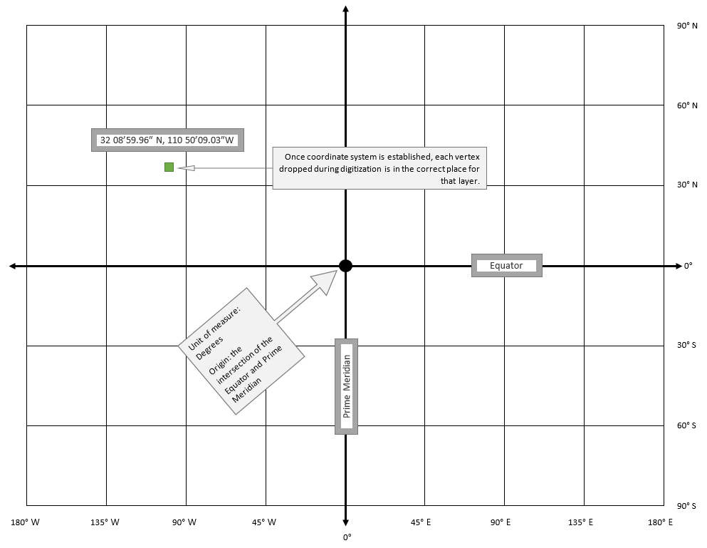 |
| All coordinate systems have a defined origin and unit of measure. Once the software is aware of the origin of the system and the unit of measure, vertices can be placed at the correct position in order to digitize new features. |
Defining the Coordinate System When It's Undefined or Fixing it When It's Incorrect
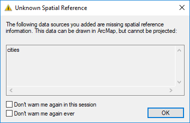
Sometimes, we add data to the software and we get a message that the layer can be added to ArcMap, but cannot be projected. This means one of two things: the coordinate system is missing, so the hidden table of vertex pl. vertices One of a set of ordered x,y coordinate pairs that defines the shape of a line or polygon feature. locations cannot establish the origin or unit of measure in which to plot said vertices OR the layer is a raster which has been scanned but not yet georeferenced. If it is the latter, the GIS Geographic Information Systems the software used to create, store, and manage spatial data Data that deals with location, such as lists of addresses, the footprint of a building, the boundaries of cities and counties, etc. , analyze spatial problems, and display the data in cartographic layouts Geographic Information Sciences technician must go through the georeferencing process to "tell" the raster layer where it "lives" in the world. If it is the former, a simple tool by the name of Define Projection can be run in order to define the coordinate system, meaning the vertices have a coordinate system origin and unit of measure to work from.
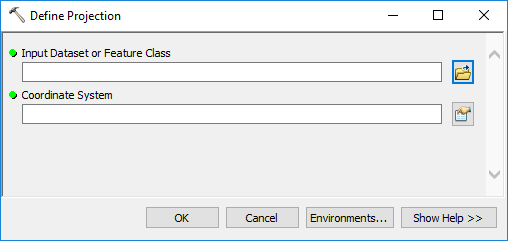
The Define Projection tool has only two jobs in the GIS Geographic Information Systems the software used to create, store, and manage spatial data Data that deals with location, such as lists of addresses, the footprint of a building, the boundaries of cities and counties, etc. , analyze spatial problems, and display the data in cartographic layouts Geographic Information Sciences : 1. define the coordinate system for a layer which contains coordinate pairs in the form of vertices (for vector layers) or an extent bounding box (for raster layers), and 2. correct the coordinate system for a layer which has been defined in a coordinate system different than the one the data was created under.
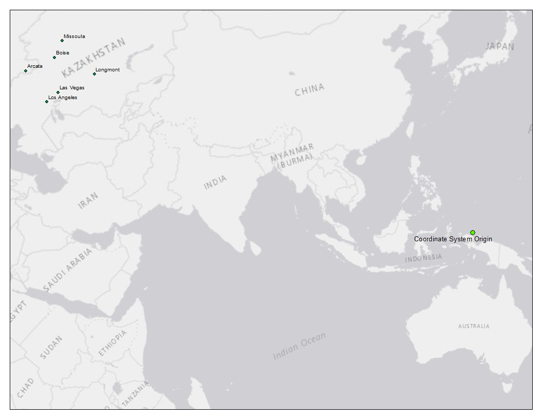
It is important to define the correct system for a layer since we know that each coordinate system has only one origin from which to start counting along the X and Y axis and only one unit of measure which defines the intervals between the horizontal and vertical lines of the X and Y axis. If a layer has been "told" that is is measuring in meters and the origin is in Central Australia when in reality it should be measuring in decimal degrees measurement of plane angle, representing 1⁄360 of a full rotation (circle). In full, a degree of arc or arc degree. Usually denoted by ° with an origin where the Equator and Prime Meridian the name of the principal meridian the north-south line from which the labeling begins. East-west lines have a very obvious start point: the equator. North-south lines must start somewhere, so when it is established for a particular geographic grid, it can be considered the principal meridian. in the latitude/longitude system meet, the resulting features are going to be very, very far off!
| Figure 6.11: Looking at the Define Tool | |
|---|---|
 |
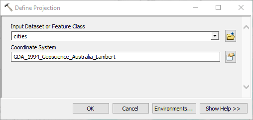 |
| When the Cities layer is added to an ArcMap session, an error is presented stating the layer can be drawn but not projected. | The Define Projection tool is run, but the wrong coordinate system is used as an input, as these cities were digitized A term to describe data which was created through the act of digitizing The action of creating vector data in any sort of digital science or art, is simply denoting a type of graphical representation using straight lines to construct the outlines of objects by defining the location of each vertex pl. vertices One of a set of ordered x,y coordinate pairs that defines the shape of a line or polygon feature. utilizing drawing pad and puck (manual or hardcopy digitizing) or a computer with a mouse (heads-up or on-screen digitizing) while, most often, looking at and tracing aerial or satellite imagery. in WGS84. |
 |
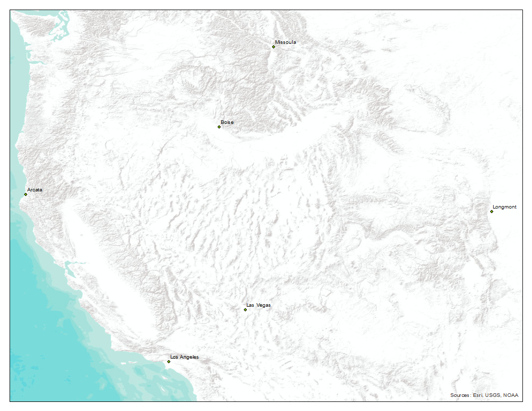 |
| The result of the Define Projection tool. ArcMap will always do exactly what you tell it to do, whether the inputs are correct or not. | After the Define Projection tool was used to correct the coordinate system, the US Cities are plotted in the correct position. |
The Project Tool
The Define Projection tool is used, as stated above, for only two tasks: setting the coordinate systems when there is not one stored with a spatial layer which should have a coordinate system established and correcting the coordinate system if an incorrect one has been defined. When the data needs to be stored in a different coordinate system, the proper tool to use is the Project tool. This tool creates a new output layer with all of the vertices moved from one coordinate system to another, and can be used to convert data from one GCS to another GCS, from a GCS to a PCS, from a PCS to a GCS, or from one PCS to another PCS. Since all coordinate systems can be correlated in the software, vertices can be moved from one system to another. It's important to understand that the coordinate system of the underlying data is actually being changed utilizing the tool and a whole bunch of hidden automagical calculus.
The need to project data from one coordinate system to another is quite important in the GIS Geographic Information Systems the software used to create, store, and manage spatial data Data that deals with location, such as lists of addresses, the footprint of a building, the boundaries of cities and counties, etc. , analyze spatial problems, and display the data in cartographic layouts Geographic Information Sciences . For example, you may collect data with a GPS Global Positioning System: A satellite-based navigation system owned and operated by the United States Department of Defense that provides location and time information anywhere on Earth. receiver in WGS84, but need to analyze the data using linear units and a projected coordinate system which preserved area. In this case, the data will need to be projected from a GSS, WGS84, to a PCS centralized on the area where the data was collected. Another example is after that data has been analyzed in the GIS Geographic Information Systems the software used to create, store, and manage spatial data Data that deals with location, such as lists of addresses, the footprint of a building, the boundaries of cities and counties, etc. , analyze spatial problems, and display the data in cartographic layouts Geographic Information Sciences with the PCS focused on area, the data might be projected again to a PCS which preserves shape in order to present the data to the client. While the projection technically: the result of using one of variety of methods to transfer the geographic locations of features from a geographic coordinate system to a developable surface everyday use: any coordinate system, geographic or projected for analysis was correct as it preserved area, the correct projection technically: the result of using one of variety of methods to transfer the geographic locations of features from a geographic coordinate system to a developable surface everyday use: any coordinate system, geographic or projected for display might be one which preserves shape.
Geographic Transformations
Before we can define what a geographic transformation The mathematical process of converting coordinates from one geographic coordinate system to another when they use different datums, accounting for differences in how Earth's shape and position are modeled. is, we need first to review a few concepts: 1. We learned in the section above that the Project tool uses automagical calculus to convert the stored coordinates of each vertex pl. vertices One of a set of ordered x,y coordinate pairs that defines the shape of a line or polygon feature. from one coordinate system to another based on internal stored tables of correlated data; 2. We learned in Chapter Two that a datum is one part of a geographic coordinate system, where a geoid a model of the variation between global mean (average) sea level and local mean sea level the measurement above or below the global average at a single point A GIS vector data in any sort of digital science or art, is simply denoting a type of graphical representation using straight lines to construct the outlines of objects geometry type which is made up of just one vertex pl. vertices One of a set of ordered x,y coordinate pairs that defines the shape of a line or polygon feature. , marking a single XY location in any given geographic or projected coordinate system. on the Earth's surface used for recording the elevation of topographic surface a detailed map of the surface features of land. It includes the mountains, hills, creeks, and other bumps and lumps on a particular hunk of earth. The word is a Greek-rooted combo of topos meaning "place" and graphein "to write." 's relief the difference between the highest and lowest point within a particular area while landforms are the descriptive words for individual features , which is used to measure precise elevations on the topographic surface a detailed map of the surface features of land. It includes the mountains, hills, creeks, and other bumps and lumps on a particular hunk of earth. The word is a Greek-rooted combo of topos meaning "place" and graphein "to write." and a reference ellipsoid an ellipsoid that is drawn to best-fit an area. World reference ellipsoids are drawn to best-fit the entire geoid; local ellipsoids are best fit on one side to a single place of the geoid are connected via control points prior to the geographic grid the result of using an established angular unit of measure to label the intersections of north-south and east-west lines on the surface of the Earth starting the labels at a principal meridian the north-south line from which the labeling begins. East-west lines have a very obvious start point: the equator. North-south lines must start somewhere, so when it is established for a particular geographic grid, it can be considered the principal meridian. being drawn upon the reference ellipsoid an ellipsoid that is drawn to best-fit an area. World reference ellipsoids are drawn to best-fit the entire geoid; local ellipsoids are best fit on one side to a single place of the geoid ; 3. Reference ellipsoids come in two varieties: global and local, where the former fits pretty okay everywhere, but super great anywhere specific and the latter fits great somewhere specific but terribly everywhere; and 4. all projected coordinate systems are based on geographic coordinate systems.
Which leads us to geographic transformations - an additional input to the Project tool which adds some specific calculus equations to assist in the conversion of XY coordinates when the input and output coordinate systems are based on different datums. This means if a layer is currently stored in the GCS WGS84, which is based on the WGS84 datum and the goal is to project it into the PCS State Plane Coordinate System - Colorado Central, which is based on the North American Datum of 1983 (NAD83), a geographic transformation The mathematical process of converting coordinates from one geographic coordinate system to another when they use different datums, accounting for differences in how Earth's shape and position are modeled. is needed, since each coordinate system is based on a different datum.
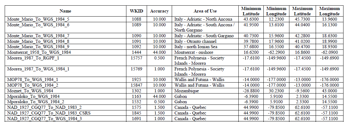
Many times when the Project tool is run, the proper geographic transformation The mathematical process of converting coordinates from one geographic coordinate system to another when they use different datums, accounting for differences in how Earth's shape and position are modeled. is offered up to the user, however, in cases where several geographic transformations could possibly apply, a filtered list will be offered up. All geographic transformations are listed in a table included with the installation of ArcGIS, and the software manufacturer assumes the GIS Geographic Information Systems the software used to create, store, and manage spatial data Data that deals with location, such as lists of addresses, the footprint of a building, the boundaries of cities and counties, etc. , analyze spatial problems, and display the data in cartographic layouts Geographic Information Sciences technician is educated in what a geographic transformation The mathematical process of converting coordinates from one geographic coordinate system to another when they use different datums, accounting for differences in how Earth's shape and position are modeled. is and how to look up the proper one when needed.
| Figure 6.12: Define Projection Tool, Project tool, and Geographic Transformations | |
|---|---|
 |
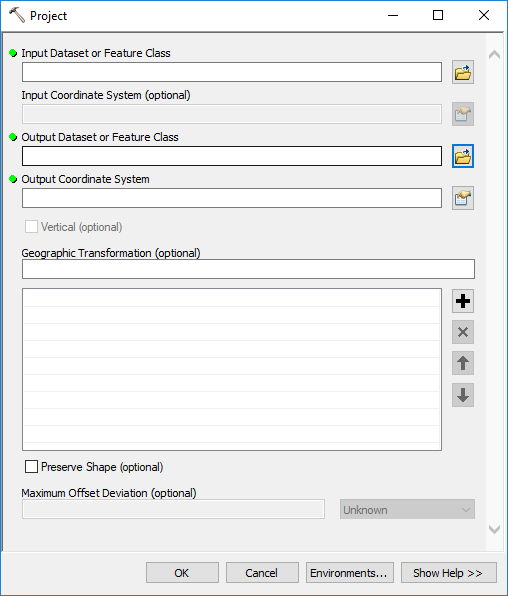 |
| The Define Projection tool has two tasks: set the coordinate system for a spatial layer when one is unknown or correcting the coordinate system when it's incorrect | The Project Tool changes the coordinate system from the one stored in the input layer to another for the output layer |
 |
|
|
A portion of the geographic transformation The mathematical process of converting coordinates from one geographic coordinate system to another when they use different datums, accounting for differences in how Earth's shape and position are modeled. table |
|
6.4.3: A Review of Selecting Data
In the next section, we are going to look at how and why we edit existing data, both the features and the associated attributes. To accomplish the task of editing existing features, we need to let the software know which feature it is we wish to edit. This designation is made by selecting the feature, as only one feature - point A GIS vector data in any sort of digital science or art, is simply denoting a type of graphical representation using straight lines to construct the outlines of objects geometry type which is made up of just one vertex pl. vertices One of a set of ordered x,y coordinate pairs that defines the shape of a line or polygon feature. , marking a single XY location in any given geographic or projected coordinate system. , polyline A GIS vector data in any sort of digital science or art, is simply denoting a type of graphical representation using straight lines to construct the outlines of objects geometry type which is made up of two or more vertices connected by straight lines. Often used to represent objects such as roads, river, and boundaries. , or polygon - can be edited at a time. In Chapter Five, we took a rather in-depth look at selecting data, so here we are just going to review the topics.
In order to edit data, we need to first select the data that needs to be edited prior to making any changes. The three main ways we select data for editing:
-
-
Interactive Selection - choose the features by clicking on the map
-
Select by Attribute- choosing features from the data set by using a SQL statement
-
Select by Location - using a spatial relationship to select the features
-
Interactive Selection
Interactive Selection is much like it sounds - highlighting features in an interactive way using a combination of the the Interactive Selection tool  in combination with a selection method. The user clicks on features in the map, which results in the desired selection. As ArcGIS only allows the user to edit one feature at a time, and frequently, the fastest way to select just one feature is interactive selection.
Select by Attribute
Select by Attribute is another method of selecting features. Using a query language called SQL, a user can create either simple or complex expressions to query (or ask) the attribute table which features meet the specified criteria, then return the result by highlighting both the rows in the attribute table and the corresponding features. As several features may be returned and ArcGIS only lets a user edit one feature at a time, utilizing the Select by Attribute's selection method options, the user can narrow down the selection to just one feature at a time. The user can also use the attribute table's "Show Selected Records" view (vs the "Show All Records") to examine the selected data, then interactively select a single feature either in the map with the Interactive Selection tool or in the attribute table using table interactive selection methods. Both of these skills have been and will continue to be practiced in lab.
Select by Location
Select by Location allows for a feature to be selected for editing based not on a value in the attribute table, but on a spatial relationship between two features in different layers, such as “select from the rivers layer all features which intersect features found in the building layer” since we would most likely want to edit river features that incorrectly flow through buildings. There is most likely no value in the attribute table which identifies a river which intersects a building, because if there was, it was probably an intentional intersection. Since there is no attribute table value to note which rivers incorrectly intersect buildings, we need to use another tool in our toolbox, and in this case, Select by Location is the best one for the job at hand.
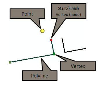
A Vertex, Vertices, and Nodes - The Building Blocks of Vector Data
We learned in Chapter Three that all vector data in any sort of digital science or art, is simply denoting a type of graphical representation using straight lines to construct the outlines of objects is made up of a series of vertices - point A GIS vector data in any sort of digital science or art, is simply denoting a type of graphical representation using straight lines to construct the outlines of objects geometry type which is made up of just one vertex pl. vertices One of a set of ordered x,y coordinate pairs that defines the shape of a line or polygon feature. , marking a single XY location in any given geographic or projected coordinate system. data is one vertex pl. vertices One of a set of ordered x,y coordinate pairs that defines the shape of a line or polygon feature. per feature, polyline A GIS vector data in any sort of digital science or art, is simply denoting a type of graphical representation using straight lines to construct the outlines of objects geometry type which is made up of two or more vertices connected by straight lines. Often used to represent objects such as roads, river, and boundaries. data is two or more vertices connected by straight lines, and polygon data is three or more vertices connected by straight lines and closed to make a shape. When data is edited, it is a process of moving or deleting existing vertices or adding additional vertices to change the look of existing features.
ArcGIS aids you when you are changing data by showing you if you are interacting with a vertex pl. vertices One of a set of ordered x,y coordinate pairs that defines the shape of a line or polygon feature. or a node, and to which particular layer it belongs. To review:
|
 |
6.4.4: Direct Feature (Map) Edits
We learned earlier in this chapter that heads-up or on-screen digitizing The action of creating vector data in any sort of digital science or art, is simply denoting a type of graphical representation using straight lines to construct the outlines of objects by defining the location of each vertex pl. vertices One of a set of ordered x,y coordinate pairs that defines the shape of a line or polygon feature. utilizing drawing pad and puck (manual or hardcopy digitizing) or a computer with a mouse (heads-up or on-screen digitizing) while, most often, looking at and tracing aerial or satellite imagery. is the process of looking at imagery and extracting vector features. In this section, we are going to take a minute to look at the process which goes into the actual creation of those features. ArcMap lumps together both new feature creation (as in, there is now a vector feature where none existed before) and feature editing (as in, the feature exists, albeit incorrect) into the same category simply named Editing. Editing, in ArcMap, also includes attribute table edits (but not new field creation, just to be confusing).
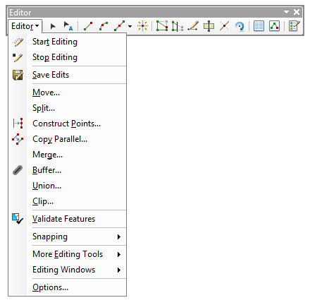
In order to let ArcMap know you'd like to either create new features or edit existing features, the first step is to initiate an edit session. Starting an edit session opens a series of tools previously grayed out, as they are only available in an edit session. As all things ArcMap, there are two ways to start an edit session: via the Editor toolbar and by right-clicking on a layer's name in the Table of Contents and selecting "Start Editing". As ArcMap only allows you to edit data which is stored in a single location, or a single workspace, at at a time, using the right-click on the layer name methods prevents confusion of data location. In other words, if you had, for example, data stored in the Results folder from GIS Geographic Information Systems the software used to create, store, and manage spatial data Data that deals with location, such as lists of addresses, the footprint of a building, the boundaries of cities and counties, etc. , analyze spatial problems, and display the data in cartographic layouts Geographic Information Sciences 101 and you were working with data stored in your Results folder from a lab in Intermediate GIS Geographic Information Systems the software used to create, store, and manage spatial data Data that deals with location, such as lists of addresses, the footprint of a building, the boundaries of cities and counties, etc. , analyze spatial problems, and display the data in cartographic layouts Geographic Information Sciences , if you started editing data from Introduction to GIS Geographic Information Systems the software used to create, store, and manage spatial data Data that deals with location, such as lists of addresses, the footprint of a building, the boundaries of cities and counties, etc. , analyze spatial problems, and display the data in cartographic layouts Geographic Information Sciences , you could not - in the same edit session, make changes to the data stored in the Intermediate folder. When you start an edit session from the Editor toolbar, you are presented with an option to select the workspace with data you'd like to edit. Right-clicking on a layer's name and selecting Start Editing bypasses the need to define a workspace, saving time and preventing you from selecting the wrong workspace if you have lots of data going at once.
| Figure 6.13: Two Methods of Starting an Edit Session in ArcMap | |
|---|---|
 |
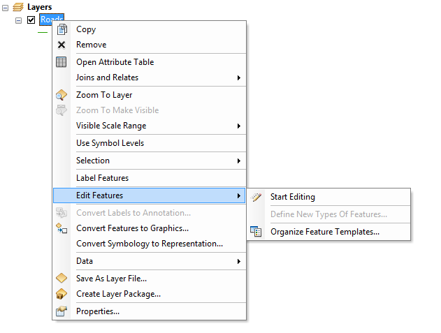 |
| Edit sessions can be launched from either the edit menu or by right-clicking on a editable layer's name and selecting "Start Editing" | |
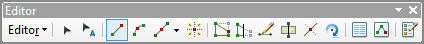
Editing Tools
As Esri has no idea what you intend to do with your data, they provide you with a variety of tools to create new features and change existing ones. As you start editing, polygon and polyline A GIS vector data in any sort of digital science or art, is simply denoting a type of graphical representation using straight lines to construct the outlines of objects geometry type which is made up of two or more vertices connected by straight lines. Often used to represent objects such as roads, river, and boundaries. layers offer some standard shapes, such as squares and rectangles, circles and ellipses, and the ability to create your own shape. As we know from Chapter Three, the definition of a vector feature is a type of graphical representation using straight lines to construct the outlines of objects, meaning that to create your own shapes (polygons and polylines), you place a series of vertices, which are automatically connected by lines. The closer those vertices are placed together, the more detail and smoothness your shapes can have. The most commonly used editing tool is the straight line tool, as that fits the definition of a vector feature. ArcGIS also provides you with some handy tools that can speed up your digitizing The action of creating vector data in any sort of digital science or art, is simply denoting a type of graphical representation using straight lines to construct the outlines of objects by defining the location of each vertex pl. vertices One of a set of ordered x,y coordinate pairs that defines the shape of a line or polygon feature. utilizing drawing pad and puck (manual or hardcopy digitizing) or a computer with a mouse (heads-up or on-screen digitizing) while, most often, looking at and tracing aerial or satellite imagery. , such as tools that automatically place lines (polylines or sides of polygons) at right angles to each other, tools which will automatically place a vertex pl. vertices One of a set of ordered x,y coordinate pairs that defines the shape of a line or polygon feature. at the midpoint of a line, Bezeir curve tools, and an actual curved line tool. It should be noted, however, that the curved line tool and the Bezeir curve tool both create a smooth, flowing shape by bending the straight line between vertices and not actually creating the line with closely placed vertices. In many instances, this may be a completely fine solution (as if it was a bad idea in every case, they wouldn't be available), but for instances when the data will be subject to topology checks, the curved lines will fail. We learned that topology is rules defining how vector features in different layers are allowed to interact with each other, such as all roads must intersect at a vertex pl. vertices One of a set of ordered x,y coordinate pairs that defines the shape of a line or polygon feature. . If a curve is present in a vector feature when it is being testing for topology, and the rules apply to that curve interacting with other features, and those other features interact not with vertices the curve is made up of (as it's made up of curved lines connecting the vertices) but the bent line of the curve, the test will fail. In order to make sure curved lines pass topology rules which include interactions and structure focused on vertices, said curves must be made out of vertices. While this may seem like a lot of if's and a very slim chance of happening, it actually happens more often than you might think. Introduction to GIS Geographic Information Systems the software used to create, store, and manage spatial data Data that deals with location, such as lists of addresses, the footprint of a building, the boundaries of cities and counties, etc. , analyze spatial problems, and display the data in cartographic layouts Geographic Information Sciences does not get into topology and topology rules, but understanding the basic concept of what topology is and roughly what it can do for us is a good starting point A GIS vector data in any sort of digital science or art, is simply denoting a type of graphical representation using straight lines to construct the outlines of objects geometry type which is made up of just one vertex pl. vertices One of a set of ordered x,y coordinate pairs that defines the shape of a line or polygon feature. , marking a single XY location in any given geographic or projected coordinate system. for future learning.
Create New Features
Create new features, as we saw previously, is the method of actually creating a new feature from scratch. Within and edit session, the Create New Features window shows all the editable layers active in your project as well as the geometries available to be added to them. By clicking the name of the layer you wish to add a feature to, the “Construction Tools” pallet opens, showing the choices available to add to that layer.
Reshape Feature
Reshape Feature allows you to select a single feature and change a portion of it, for example, if you have a river that shows it is flowing right through a building and you can see in the imagery it actually flows to the south of that building, you can select that river and use the Reshape Feature tool to draw along the actual path to get people out of “harms way”.
Edit Vertices
Edit Vertices is a tool that allows you to move or delete one or more existing vertices, as well as add new vertices to the feature. For example, if you have a road that is in the correct place, but the previous technician represented a pretty steep curve with just a few vertices, you can add a few more then move them into place to create the best line representation possible.
Editing Aids
When it comes to editing, ArcGIS provides us with several aids to guide the editing tools to produce a better product.
Snapping
How is it you know when you have connected features perfectly together? While zooming in super far is one way, it is not the most efficient way. And not always accurate either.
This is where snapping comes in. Snapping is a feature built into the GIS Geographic Information Systems the software used to create, store, and manage spatial data Data that deals with location, such as lists of addresses, the footprint of a building, the boundaries of cities and counties, etc. , analyze spatial problems, and display the data in cartographic layouts Geographic Information Sciences where your cursor jumps or ‘snaps’ to a vertex pl. vertices One of a set of ordered x,y coordinate pairs that defines the shape of a line or polygon feature. . If you think of snapping your coat, where half of the snap lines itself up with the other half via the concave surface, snapping in the GIS Geographic Information Systems the software used to create, store, and manage spatial data Data that deals with location, such as lists of addresses, the footprint of a building, the boundaries of cities and counties, etc. , analyze spatial problems, and display the data in cartographic layouts Geographic Information Sciences is very similar. After setting a ‘snapping tolerance’, or the distance away from a vertex pl. vertices One of a set of ordered x,y coordinate pairs that defines the shape of a line or polygon feature. where you’d like your cursor to automatically jump (think the outer edge of the coat snap - as long as you get the snap near the edge of the receiver end, it will line itself up and snap into place), you can use snapping to be perfectly sure your features are meeting exactly.
Tracing
Tracing is another available ‘helper’ feature built in to map edits. Tracing allow you to exactly follow a path of an existing vector feature. (This is not like ArcScan that traces raster into vectors) Trace allow you easily and correctly complete tasks such as collecting a line feature that must meet exactly with polygon feature, creating a polygon that must meet another polygon, or using the trace offset to create a feature that is exactly the same but some distance away, for example, two parallel roads 50 feet apart.
6.4.5: Attribute Table Edits
In GIS Geographic Information Systems the software used to create, store, and manage spatial data Data that deals with location, such as lists of addresses, the footprint of a building, the boundaries of cities and counties, etc. , analyze spatial problems, and display the data in cartographic layouts Geographic Information Sciences 101 labs, attribute tables for the data used are almost always neatly populated with the data needed, and you can assume that data is correct - that is unless the task in lab is to create attributes or correct attributes, both of which would be neatly outlined in the instructions. Beyond GIS Geographic Information Systems the software used to create, store, and manage spatial data Data that deals with location, such as lists of addresses, the footprint of a building, the boundaries of cities and counties, etc. , analyze spatial problems, and display the data in cartographic layouts Geographic Information Sciences 101 (well, and during lab sessions in GIS Geographic Information Systems the software used to create, store, and manage spatial data Data that deals with location, such as lists of addresses, the footprint of a building, the boundaries of cities and counties, etc. , analyze spatial problems, and display the data in cartographic layouts Geographic Information Sciences 101) making Attribute Table edits are extremely important. Unlike direct feature edits, ArcMap allows a user to edit the attribute table both within and outside of an edit session, the two main differences being edits inside an edit session do not rely solely on a tool to make the changes and those edits can be undone if a mistake is made. Outside an edit session, the attribute table table changes, made only via the Field Calculator or Calculate Geometry tools, cannot be undone. Hopefully there is a copy of the data or it's easy to put back all the incorrect values!
Direct Record Editing
In an edit session, each value in an attribute table can be edited independently of the other values by clicking inside the cell, deleting the contents, and entering a new value, just like on would do using Microsoft Excel or OpenOffice Calc. This is the easiest way to correct or change just a few values, however, this method also can create unintended error in the attribute table, since we know that “Kalifornia” and “California” are not the same value (that's an example of a pretty obvious error, but missing a letter while typing is actually quite likely). To populate more than one record at a time and assure the values are perfectly identical, we use the attribute table tool, Field Calculator.
Field Calculator
Field Calculator is an attribute table tool which can populate, change, or clear records within a single field for either selected records (selected via attribute, location, or interactive selection) or all records. It's capable of populating records with either integers, decimal numbers, text, or time/date, depending on the field type as the result of establishing a single value for the desired records or the result of a mathematical calculation between two records, a record and a value, or two values (all of these include the words "or more", as the calculation is not limited to just two items). These mathematical calculations can be between numbers or letters, as long as the two items are a match type.
If the goal was to add two fields together, one field containing “FLOOD_RISK” values and the other containing “FIRE_RISK” values, to find the “TOTAL_RISK”. By combining an assessed value for flood risk with an assessed value of fire risk, you can determine the total risk for a entire neighborhood which could be used for insurance premiums or deciding where to spend a federal grant. Using the Field Calculator, you can create the mathematical equation of “FLOOD_RISK” + “FIRE_RISK” to find "TOTAL_RISK". The tool will automatically add the Flood Risk for a single feature to the Fire Risk of that same feature. For example, if the task is to find the Total Risk for each parcel in a county and each parcel row contains a flood and a fire risk value, Field Calculator will add the risk associated with each parcel.
| Figure 6.14: Field Calculator Example of Adding Fields |
|---|
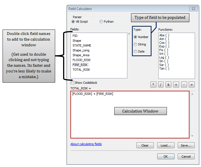 |
| Field Calculator can be used to complete mathematical calculations (add, subtract, multiply, divide, and advanced methods) between the values contained in two or more fields, as long as those fields are of the same type. |
It is also possible to "add" two text fields together, concatenating the values. For example, if one field contained the house numbers and another field contained the street names, those field can be added together with the goal of creating a new field which contained the entire street address. As long as all the fields in the equation are of the same type (integer, decimal, text, or date), they can participate in a Field Calculator equation.
|
We learned earlier that the text field type will accept number and date records, but only number fields will treat the characters like numbers, putting them in numeric order 1 - 2 - 10 - 20 - 110 - 220, vs "alphabetizing" them 1 - 10 - 110 - 2 - 20 - 220, and only date fields treat the values like dates, putting them in calendar order vs alphabetizing them. |
Calculate Geometry
The other field calculation tool we use in ArcGIS is Calculate Geometry, which has the single task of populating fields with area, length, or coordinate pairs. For the point A GIS vector data in any sort of digital science or art, is simply denoting a type of graphical representation using straight lines to construct the outlines of objects geometry type which is made up of just one vertex pl. vertices One of a set of ordered x,y coordinate pairs that defines the shape of a line or polygon feature. , marking a single XY location in any given geographic or projected coordinate system. geometry type, the only available item to calculate is the XY coordinate pair in either a geographic or projected coordinate system. For polygons, the coordinate pair of the perfect center of the polygon can be found, while the coordinate pairs of the center and ends of a polyline A GIS vector data in any sort of digital science or art, is simply denoting a type of graphical representation using straight lines to construct the outlines of objects geometry type which is made up of two or more vertices connected by straight lines. Often used to represent objects such as roads, river, and boundaries. can be found FYI, there are tools outside of Calculate Geometry, which is a single field attribute table tool, that can find the coordinate pair for all of the vertices for polylines, polygons.
Areas of polygons and lengths of both polylines and the perimeter of polygons can also be found, both in angular and linear units using the Calculate Geometry tool. This would comes in handy, as one example, after a series of geoprocesses have been run and the total area or length would need to be reported.
The Calculate Geometry is capable of solving areas, lengths, and coordinate pairs in both the coordinate system the layer is stored in as well as the coordinate system the data frame is in. If your layer is saved in a different coordinate system, it’s advised to give the field a heading which included measurement units, such as Area_FEET, since attribute tables never include units.