When we add external data tables to spatial data, our ability to solve spatial problems increases exponentially. External data tables not only store an entire history of pre- GIS Geographic Information Systems the software used to create, store, and manage spatial data, analyze spatial problems, and display the data in cartographic layouts Geographic Information Sciences data, but can also store data which would otherwise be extraneous, depending on the specific GIS Geographic Information Systems the software used to create, store, and manage spatial data, analyze spatial problems, and display the data in cartographic layouts Geographic Information Sciences project. If you wanted to create one shapefile One of the two main types of vector data in any sort of digital science or art, is simply denoting a type of graphical representation using straight lines to construct the outlines of objects we learn in this class (there are more than two vector data in any sort of digital science or art, is simply denoting a type of graphical representation using straight lines to construct the outlines of objects types in GIS). Shapefiles are each only one geometry type, either a point, a polyline, or a polygon. Shapefiles are stored in folders and most often do not have relationships with other data. with all of the data that could possibly be stored about one location, the result would be a huge, unmanageable file that would probably still be missing data that you didn’t think of. External tables relieves this “ shapefile One of the two main types of vector data in any sort of digital science or art, is simply denoting a type of graphical representation using straight lines to construct the outlines of objects we learn in this class (there are more than two vector data in any sort of digital science or art, is simply denoting a type of graphical representation using straight lines to construct the outlines of objects types in GIS). Shapefiles are each only one geometry type, either a point, a polyline, or a polygon. Shapefiles are stored in folders and most often do not have relationships with other data. congestion” by allowing data to be stored outside the GIS Geographic Information Systems the software used to create, store, and manage spatial data, analyze spatial problems, and display the data in cartographic layouts Geographic Information Sciences until it is needed. When it is needed, we connect it back to GIS Geographic Information Systems the software used to create, store, and manage spatial data, analyze spatial problems, and display the data in cartographic layouts Geographic Information Sciences data via a join or relate.
The idea of joining and relating data allows us to have a large quantity of data for an area without having large shapefiles or feature classes. Depending on the geoprocessing tool you are running, the process time can increase based on the number of fields, even if the tool isn't dealing with those extraneous fields. To keep file size low and processing time down, we can join and relate non-spatial data Attributes related to a location but not describing its physical placement in space, such as information about a tree's age, type, and health. tables back to a specific shapefile One of the two main types of vector data in any sort of digital science or art, is simply denoting a type of graphical representation using straight lines to construct the outlines of objects we learn in this class (there are more than two vector data in any sort of digital science or art, is simply denoting a type of graphical representation using straight lines to construct the outlines of objects types in GIS). Shapefiles are each only one geometry type, either a point, a polyline, or a polygon. Shapefiles are stored in folders and most often do not have relationships with other data. or feature class One of the two main types of vector data in any sort of digital science or art, is simply denoting a type of graphical representation using straight lines to construct the outlines of objects we learn in this class (there are more than two vector data in any sort of digital science or art, is simply denoting a type of graphical representation using straight lines to construct the outlines of objects types in GIS). Feature classes are each only one geometry type, either a point A GIS vector data in any sort of digital science or art, is simply denoting a type of graphical representation using straight lines to construct the outlines of objects geometry type which is made up of just one vertex pl. vertices One of a set of ordered x,y coordinate pairs that defines the shape of a line or polygon feature. , marking a single XY location in any given geographic or projected coordinate system. , a polyline A GIS vector data in any sort of digital science or art, is simply denoting a type of graphical representation using straight lines to construct the outlines of objects geometry type which is made up of two or more vertices connected by straight lines. Often used to represent objects such as roads, river, and boundaries. , or a polygon. Feature classes are stored in geodatabases and are most often used when data relationships are important. .
Imagine you are city GIS Geographic Information Systems the software used to create, store, and manage spatial data, analyze spatial problems, and display the data in cartographic layouts Geographic Information Sciences manager. You have tons of data about your city, and every intern season even more is collected. Your interns collect data about street damage, sign locations, tree health, bike lane usage, building exterior condition, zoning types, and on and on and on. All of this data has value and is important to different projects throughout the year, so you wouldn't want to delete any of it. Yet, on the other hand, it is too much data to deal with at any one time. If you created one giant shapefile One of the two main types of vector data in any sort of digital science or art, is simply denoting a type of graphical representation using straight lines to construct the outlines of objects we learn in this class (there are more than two vector data in any sort of digital science or art, is simply denoting a type of graphical representation using straight lines to construct the outlines of objects types in GIS). Shapefiles are each only one geometry type, either a point, a polyline, or a polygon. Shapefiles are stored in folders and most often do not have relationships with other data. of building and created fields for every possible bit of data you know about your buildings (color, material, zoning, address, occupants, real estate history, ...) you would have one huge shapefile One of the two main types of vector data in any sort of digital science or art, is simply denoting a type of graphical representation using straight lines to construct the outlines of objects we learn in this class (there are more than two vector data in any sort of digital science or art, is simply denoting a type of graphical representation using straight lines to construct the outlines of objects types in GIS). Shapefiles are each only one geometry type, either a point, a polyline, or a polygon. Shapefiles are stored in folders and most often do not have relationships with other data. ! To keep sizes small, we use joins and relates to connect our non-spatial data Attributes related to a location but not describing its physical placement in space, such as information about a tree's age, type, and health. tables to our spatial data when we need it, leaving it as separate tables when we don't.
Many organizations which serve up data on the internet, such as US Census data and water monitoring projects, store and allow for data download in this format. One file will contain the spatial data and the other will be a non-spatial table, and you will be expect to join the two in ArcGIS.
5.10.2: Table Joins vs Relates
Joins and relates are really quite similar in their function: the ability to include additional data for a shapefile One of the two main types of vector data in any sort of digital science or art, is simply denoting a type of graphical representation using straight lines to construct the outlines of objects we learn in this class (there are more than two vector data in any sort of digital science or art, is simply denoting a type of graphical representation using straight lines to construct the outlines of objects types in GIS). Shapefiles are each only one geometry type, either a point, a polyline, or a polygon. Shapefiles are stored in folders and most often do not have relationships with other data. or feature class One of the two main types of vector data in any sort of digital science or art, is simply denoting a type of graphical representation using straight lines to construct the outlines of objects we learn in this class (there are more than two vector data in any sort of digital science or art, is simply denoting a type of graphical representation using straight lines to construct the outlines of objects types in GIS). Feature classes are each only one geometry type, either a point A GIS vector data in any sort of digital science or art, is simply denoting a type of graphical representation using straight lines to construct the outlines of objects geometry type which is made up of just one vertex pl. vertices One of a set of ordered x,y coordinate pairs that defines the shape of a line or polygon feature. , marking a single XY location in any given geographic or projected coordinate system. , a polyline A GIS vector data in any sort of digital science or art, is simply denoting a type of graphical representation using straight lines to construct the outlines of objects geometry type which is made up of two or more vertices connected by straight lines. Often used to represent objects such as roads, river, and boundaries. , or a polygon. Feature classes are stored in geodatabases and are most often used when data relationships are important. to increase the ability to solve spatial problems, examine additional associated data, and symbolize a map based on different criteria. The main difference between them lies with the result of the tool: joined tables append additional fields while relates leave the data where it's at, simply showing the user the associated data between tables. There are other, smaller differences as outlined below:
| Table Joins | Relates |
|---|---|
|
|
| Figure 5.17: Joins Vs Relates |
|---|
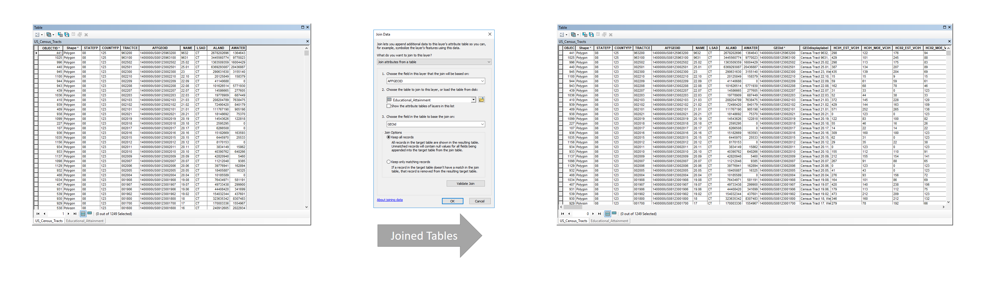 |
| Joined tables. After the join action is performed between the US Census tract shapefile One of the two main types of vector data in any sort of digital science or art, is simply denoting a type of graphical representation using straight lines to construct the outlines of objects we learn in this class (there are more than two vector data in any sort of digital science or art, is simply denoting a type of graphical representation using straight lines to construct the outlines of objects types in GIS). Shapefiles are each only one geometry type, either a point, a polyline, or a polygon. Shapefiles are stored in folders and most often do not have relationships with other data. and the Educational Attainment non-spatial data Attributes related to a location but not describing its physical placement in space, such as information about a tree's age, type, and health. table, the fields from the Educational Attainment |
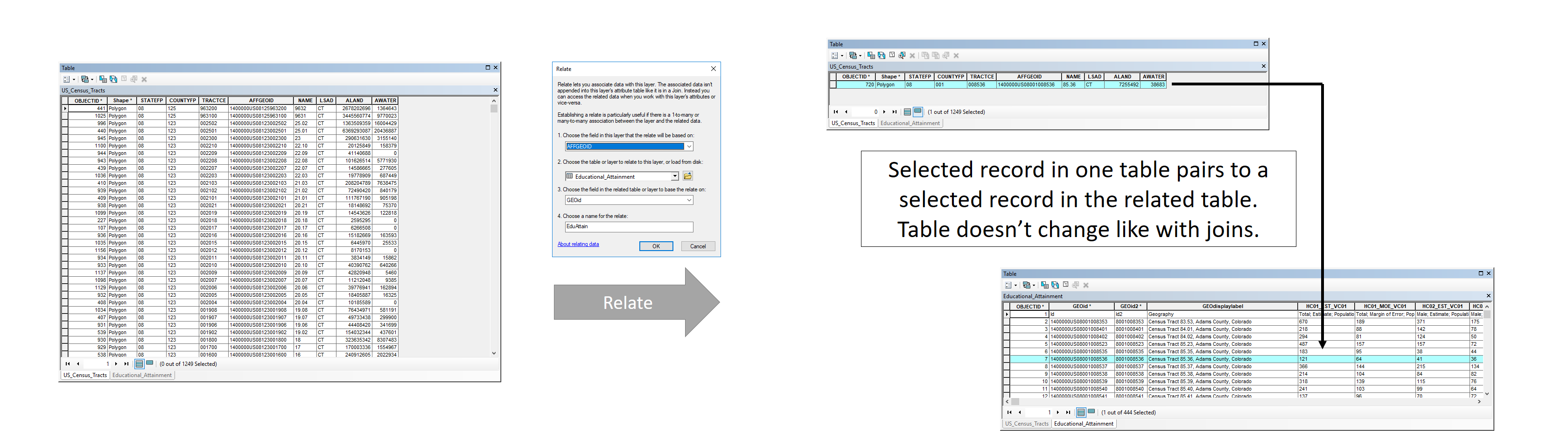 |
| Related tables. Related tables are bi-directional, meaning that to find the related features/rows in one layer/non-spatial table is to select features in the other and use the "Related Feature" button to select the corresponding row in the other layer/non-spatial table. |
5.10.3: Keys
As table joins append field and relates leave the tables as it, we know that both table joins and relates are a table-based operation, meaning that these two processes rely on a key or common value between both tables. This common value is the item which ties each table together, whether that's to append the fields in a table join or relate the tables with a relate.
Key values have two mandatory requirements to consider them key values - they must be stored in fields of the same type (string, float, double, integer, date) in each table and they must be the exact same value, character for character, space for space (spaces when applicable). This means that if the table join or relate is intended to be completed on a string value, the field must be string in both table, regardless if they are letters or numbers within that field. If the table join or relate is intended to be completed on a float, double (both decimal number values), short integer, long integer (whole numbers without a decimal), or date, the field in each table must both be of a matching type.
| Figure 5.18: An Example of Key Value in Two Tables | |
|---|---|
 |
|
Matching records, or the identical value in both tables, must also be, as stated above, must be identical character for character in both tables. This means that the value "colorado" in Table A will NOT match to the value "Colorado" in Table B. The fact that Colorado is capitalized on one table and not in the other means they are not the same value, character for character. Another example of what would not join is the value 085548375 and 85548375, as the leading zero makes the first value different from the second.
Two items that don't matter when it comes to table joins and relates are what the field is actually called and how many values are in the field. As long as you know the values contained in the field are exactly the same, it makes no difference what the field is called, as well as how many will be matching records. A table join or relate may be completed on one value or thousands of values. In addition, the number of values do not need need to match in both tables. Just like it doesn't matter the number of matching records, the number of values in both tables do not need to match. One field can contain 27 values, the other can contain 420 values, and only 5 of those values can successfully match and it makes no difference.
One thing that should be noted when it comes to table joins and relates is the fact that these are almost never completed on the OID (object identifier) or the FID (feature identifier). We learned in the section about databases that each table contains at least one unique value per row, and we call that row the OID or FID. These values are, in general, completely random. When tables are created, the OID or FID are populated as each row is added. For example, if you intend to keep the FID in a particular order while digitizing The action of creating vector data in any sort of digital science or art, is simply denoting a type of graphical representation using straight lines to construct the outlines of objects by defining the location of each vertex pl. vertices One of a set of ordered x,y coordinate pairs that defines the shape of a line or polygon feature. utilizing drawing pad and puck (manual or hardcopy digitizing) or a computer with a mouse (heads-up or on-screen digitizing) while, most often, looking at and tracing aerial or satellite imagery. a series of roads and you skip one on accident, in order to keep the data complete (Chapter Eight), you will need to go back digitize that missing road. The series of values in the FID field will continue where it left off and your intended series of values will be broken. The solution? Create a field where a value is associated with each road, just like the player ID we saw in the database electronic storage container with a top-down structure in which the items contained are related to each other and that relationship allows for the data to be quickly and efficiently queried and retrieved for use. example. This value will have nothing to do with the FID, meaning you can go back and complete things like table joins, relates, and select by attribute based on this value.
5.10.4: Data Relationships
Once a key is established in a table join or relate, the next step is to establish a relationship - one-to-one, one-to-many, many-to-one, and many-to-many. In ArcMap, this relationship is often implied based upon which tables are chosen to be joined and the order in which they are joined - that is to say the relationship is determined by ArcMap based upon which table goes first in the table join tool and which table goes second. Relates are bi-directional since the fields are not appended, the software just shows the related field in each table via highlighting them. The relationship type still exists, but there isn't a specific need to establish it, since nothing is being altered in the tables. Lab will explore this idea, placing one table first in the tool and examining the result, then flipping the tool, putting the second table first and examining that result. This data exploration will help solidify the idea of implied relationships in ArcGIS.
Even though these relationships are implied with table joins and relates, it is still important to understand the types of table relationships, as there are some (non-101) tools which require you to establish the desired relationship yourself as well as understanding the results of the table joins completed in Introduction to GIS Geographic Information Systems the software used to create, store, and manage spatial data, analyze spatial problems, and display the data in cartographic layouts Geographic Information Sciences .
One-to-One
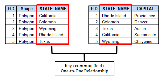
In a one-to-one relationship (seen in the image above), each feature has only one matching value based upon the selected key, (and thus one row). For example, if you were to join a state capitals data table with a states layer, each state would have only one capital, and each capital would associate with only one state.
Many-to-One
|
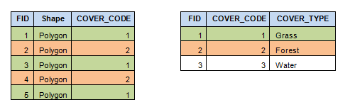
The Many-To-One Relationship are between several features and one row in a data table. The example seen the the image to the right shows a feature layer (aka a vector file, a layer with features) with two different cover codes, as designated with a coded value. The table which is being joined contains both the coded and "decoded" values (we don't really used the word 'decoded', but instead 'matched'. I didn't, however, want to confuse use by using the word 'matched' in relation to the the result of the join and the coded/decoded values - which I just did, but at least it came with an explanation the second time). |
 |
One-to-Many
|
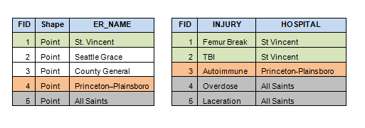
One-To-Many Relationships have a single feature which relates to two or more rows in a data table. Some non-spatial examples are: one person can play many positions on a baseball team, one person can own two (or more) cars, or many visitors visit one emergency room (which can also be a spatial relationship!). Spatial examples might be, one state can have several counties (Colorado has 64 counties) and one water sampling location has many samples. Fictitious water sampling station A342 has hourly samples taken, which are averaged together and contained in a table which shows daily, weekly, and monthly sample average along side the hourly sample taken. |
 |
Many to Many
|
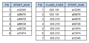
Many-To-Many are relationships where two or more features match to two or more rows in the data table. A non-spatial example of a many-to-many relationship is the academic roster of the college. Many students take many classes, which means if you were to query the database electronic storage container with a top-down structure in which the items contained are related to each other and that relationship allows for the data to be quickly and efficiently queried and retrieved for use. that holds student records, one student will return many records ( GIS Geographic Information Systems the software used to create, store, and manage spatial data, analyze spatial problems, and display the data in cartographic layouts Geographic Information Sciences 101, GIS Geographic Information Systems the software used to create, store, and manage spatial data, analyze spatial problems, and display the data in cartographic layouts Geographic Information Sciences 210, GIS Geographic Information Systems the software used to create, store, and manage spatial data, analyze spatial problems, and display the data in cartographic layouts Geographic Information Sciences 212, etc) and one course will return several students ( GIS Geographic Information Systems the software used to create, store, and manage spatial data, analyze spatial problems, and display the data in cartographic layouts Geographic Information Sciences 101: Mary Kay, Hello Kitty, Sailor Moon, etc). A spatial example of a many-to-many relationship would be speed limits and road names. Many times, as you drive along on physical road (the geometry of the road), it will change names and speed limits several times |
 |
5.10.5: Initiating, Validating, and Retaining Table Joins
So far, we've looked at what table joins and relates are, what a key is and it's requirements, and four types of table relationships. In this section, we are going to take a minute to note how we initiate a table join or relate, what validating a table join or relate does, and what happens after a successful table join. Again, this isn't for you to memorize right now, but instead to have you quickly look at how we perform table joins and relates, what and why we would want to validate said table join or relate before the actual action occurs, and what to expect after a successful table join. All of these skills will be practiced and solidified in lab, but it's a good idea to take a quick look at the process prior to lab to understand what is happening with this particular ArcGIS tool.
| The Layer Options Menu and the Layer Properties Window |
|---|
|
In ArcMap, we will interact with several "Something Options" menus, named based on the place from which the menu is launched. We looked at the Table Options menu earlier in the chapter, which was a menu launched from an attribute table and containing actions which affect an entire table. We will look a a few more throughout the text and in lab, and one of those is the Layer Options menu - a menu launched by right-clicking on a layer's name in the Table of Contents which contains actions that affect the individual layer. Examples included: adding labels to the map for that specific layer, opening the attribute table for that layer, exporting selected features to a new shapefile One of the two main types of vector data in any sort of digital science or art, is simply denoting a type of graphical representation using straight lines to construct the outlines of objects we learn in this class (there are more than two vector data in any sort of digital science or art, is simply denoting a type of graphical representation using straight lines to construct the outlines of objects types in GIS). Shapefiles are each only one geometry type, either a point, a polyline, or a polygon. Shapefiles are stored in folders and most often do not have relationships with other data. or feature class One of the two main types of vector data in any sort of digital science or art, is simply denoting a type of graphical representation using straight lines to construct the outlines of objects we learn in this class (there are more than two vector data in any sort of digital science or art, is simply denoting a type of graphical representation using straight lines to construct the outlines of objects types in GIS). Feature classes are each only one geometry type, either a point A GIS vector data in any sort of digital science or art, is simply denoting a type of graphical representation using straight lines to construct the outlines of objects geometry type which is made up of just one vertex pl. vertices One of a set of ordered x,y coordinate pairs that defines the shape of a line or polygon feature. , marking a single XY location in any given geographic or projected coordinate system. , a polyline A GIS vector data in any sort of digital science or art, is simply denoting a type of graphical representation using straight lines to construct the outlines of objects geometry type which is made up of two or more vertices connected by straight lines. Often used to represent objects such as roads, river, and boundaries. , or a polygon. Feature classes are stored in geodatabases and are most often used when data relationships are important. , and initiating table joins and relates. A list of all the functions available can be seen here: https://vector.geospatial.science/ArcMap/Layer-Options. The Layer Properties window, launched from the Layer Options menu, contains properties about each spatial layer, such as where the layer is stored on the computer, what coordinate system the layer is stored in, what the layer looks like in ArcMap, and how labels are generated. While labels can be turned on and off in the Layer Options menu, how the labels look (aka, how the labels are generated by the software) is controlled in the Layer Properties window. Overall, the Layer Options menu and the Layer Properties window are the two that technicians interact with the most within the ArcMap software. Making changes with how the layer looks and acts within the software and knowing about the properties of the layer are some of the most important things that a technician can do to make the best decisions within the software. |
Initiating Relates and Table Joins
Table Joins and Relates are initiated in one of three ways: from the Layer Options menu, from the Table Options menu within the attribute table, and from the Layer Properties window. All three methods generate the same result, with the two tables (either two attribute tables, one attribute table and one non-spatial table, or two non-spatial tables) either being appended (table joins) or related (relates). While relates are bi-directional and it really doesn't matter which one the relate is initiated from since the result is the same when it comes to highlighting features in one or the other table, joins, on the other hand, requires the user to initiate the join from the layer where the desired fields are to be appended.
In section 5.9.4, we looked at the four kinds of table relationships, where it was stated that ArcMap assumes the relationship for table joins. This assumption comes from which table the join is initiated from. It was also said that the fields which make up the joined from table (attribute or non-spatial) are the ones which will be appended to the joined to table (attribute or non-spatial). Looking at these two ideas, we can say that the table relationship is determined based on which of the layer or non-spatial table the join is initiated from. It isn't mandatory to join a non-spatial table to spatial layer, as the assumed table relationship may end up "backwards" if the join is initiated from the wrong place. It should be noted, along with the fact that it isn't mandatory to initiate a table join from a spatial layer to a non-spatial layer, that the resulting data type of a table join is equal to whichever data type the table join is initiated from. That is to say if a table join is initiated from a spatial layer, such as a point A GIS vector data in any sort of digital science or art, is simply denoting a type of graphical representation using straight lines to construct the outlines of objects geometry type which is made up of just one vertex pl. vertices One of a set of ordered x,y coordinate pairs that defines the shape of a line or polygon feature. , marking a single XY location in any given geographic or projected coordinate system. , the result of the join will continue to be a point A GIS vector data in any sort of digital science or art, is simply denoting a type of graphical representation using straight lines to construct the outlines of objects geometry type which is made up of just one vertex pl. vertices One of a set of ordered x,y coordinate pairs that defines the shape of a line or polygon feature. , marking a single XY location in any given geographic or projected coordinate system. layer. If a join is initiated from a non-spatial table, the result of the table join will continue to be a non-spatial data Attributes related to a location but not describing its physical placement in space, such as information about a tree's age, type, and health. table, with the fields from the other layer, whether that is a spatial layer or non-spatial data Attributes related to a location but not describing its physical placement in space, such as information about a tree's age, type, and health. table.
This section has looked at several ideas, some of them quite specific, like how to launch the table join and relate tool, but those skills and specifics will come in time with practice in lab. For now, it's important to understand just a few of the things we are looking at in regards to table joins: 1. the four table relationship types, 2. that table joins append fields in the joined from table (attribute or non-spatial) to the joined to table (attribute or non-spatial, and 3. that ArcMap assumes that table relationship type based on what kind of records are contained in both tables participating in the join. Know which table relationship is assumed and what the resulting join looks like are things where understanding comes in time with experience.
| Figure 5.19: Launching the Table Join and Relate tools |
|---|
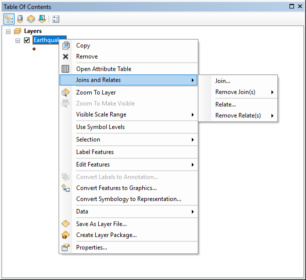 |
| Launching Join or Relate from the Table of Contents |
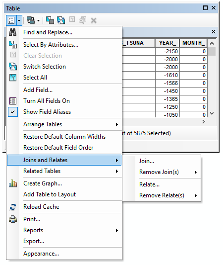 |
| Launching the Join or Relate tool from the Table Options menu in the attribute table. |
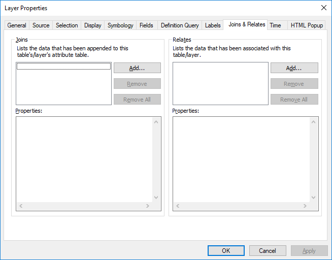 |
| Launching the Join or Relate tools form the Layer Properties window |
Validating Joins
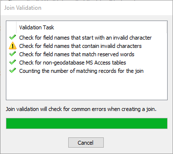
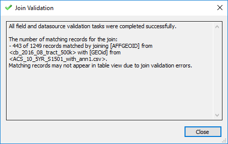
Similar to what we saw with the "Validate" button associated with SQL expression, the table join dialog box has a means of validating certain required parameters of the tool and generating a report of it's findings. This validation task checks for errors in the tables which may prevent the join from either happening at all or happening in a complete manner. The validation report shows the findings, allowing the user to go and correct any mistakes to prevent any potential errors with the join. Unlike other ArcMap errors, like the SQL error of "invalid syntax", the table join validation report is actually specific and rather helpful.
The report, specifically, is checking for invalid characters at the start of or within the field names, looking for fields names which are using reserved words, or words that are specific to how database electronic storage container with a top-down structure in which the items contained are related to each other and that relationship allows for the data to be quickly and efficiently queried and retrieved for use. tables operate and should be used in other fields which do not serve the database electronic storage container with a top-down structure in which the items contained are related to each other and that relationship allows for the data to be quickly and efficiently queried and retrieved for use. 's pre-determined purpose, and counts up how many features/rows match between the two tables.
| Figure 5.20: Table Join Validate Tool and Validation Report | |
|---|---|
 |
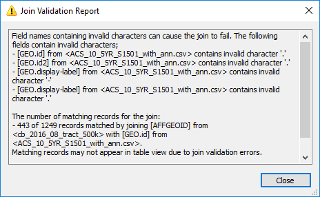 |
| Running the Join Validation tool. We seen green check marks where the tool was successful and yellow exclamation marks where there may be an error that need to be addressed. Red X's will show if there is an error which will not allow the join to occur at all. The green check mark, yellow exclamation mark, and red X theme is held throughout all geoprocessing tools in ArcGIS, not just the join validation | The Join Validation Report. This report notes that the field GEO.id, GEO.id2, and GEO.display-label all have invalid characters in their field names. these are the default field names when data is downloaded from the US Census website and even though a successful join may happen, the field names should still be corrected in Microsoft Excel or similar spreadsheet software. If you are unsure of how many records were supposed to join and you have invalid field names, and unexpected join may occur and you would never know. The easiest method to prevent any unexpected join behavior is to adjust the invalid field names in a spreadsheet software. |
 |
 |
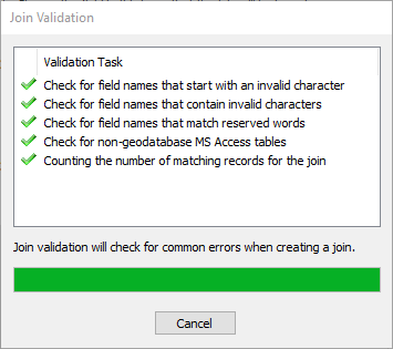
| After the field names have been corrected in Microsoft Excel, the validation tasks all report a green check mark. | The validation report shows the successful join. |
Retaining Spatial Joins and Relates
5.10.6: Preparing Data for Relates and Table Joins
When we are getting ready to perform a relate or table join, we must first make sure our data is ready to be related or joined. Sometimes, this process can be rather tedious, assuring all the field headers are in the correct format (no spaces, no special characters, not more than 10 alphanumeric characters), as well as making sure the attributes of the key are identical, since we already know that attribute tables do not tread “california” and “California” as the same value. When preparing data for relates and joins, it is often easier to adjust the values of the non-spatial data Attributes related to a location but not describing its physical placement in space, such as information about a tree's age, type, and health. table directly in Microsoft Excel then trying to edit values of the layer to which you plan to join the data. If you are joining or relating two spatial layers together, it's important NOT to use Excel to adjust the table, but to use ArcMap and the attribute table tools which you will master during lab. If you are completing a Spatial Join, there is no need to adjust anything in either of the tables to make the join work, as spatial joins are based on spatial relationships and not table values/keys. As of right now, the only real take-away from this section is that sometimes, data is not ready to be table joined or related and adjustments should/must be made prior to using the tool. Non-spatial tables are the easier of the two (vs spatial layers) to adjust prior to a table join or relate and the easiest way to do so is to use a spreadsheet software such as Microsoft Excel.
5.10.7: Spatial Joins
Thus far, we keep using the term "table join" and you may have noticed that in the picture of the tool in Figure 5.18, the tool actually says "Join" and not "Table Join". There is another tool that we use in ArcGIS called spatial join (the actual name, not an addition to the word join). Just like we have two tools for selecting features in a non-spatial and spatial way, select by attribute and select by location, we have two tools to join features, one non-spatial and one spatial. In this section, we've spent quite a bit of time looking at the non-spatial method of "table joins", which are not their real names, that is simple "join". Adding "table" to the join will help designate the non-spatial method from the spatial method.
The big difference between Select by Attribute and Select by Location is select by attribute uses the values contained in the attribute table while select by location relies on selecting features based on their relationship with each other. Select by Attribute is a non-spatial method, utilizing those values while Select by Location is a spatial method, utilizing the actual features. The big difference between table joins and spatial joins is table joins are non-spatial, utilizing the values contained in the attribute table or non-spatial data Attributes related to a location but not describing its physical placement in space, such as information about a tree's age, type, and health. table, while spatial joins utilize the actual features and their relationship with each other.
The tool uses the same spatial relationships we looked at on the Select by Location page to append fields from one layer with features in another layer, automatically producing a new output layer, not a temporary join like table joins. Since Spatial Join uses a spatial relationship, such as intersect, there is no way to complete a spatial join between a spatial layer and a non-spatial table - a noted difference between spatial joins and table joins. An example of a spatial join might be between a zip code polygon layer which has a field for the zip code and a city point A GIS vector data in any sort of digital science or art, is simply denoting a type of graphical representation using straight lines to construct the outlines of objects geometry type which is made up of just one vertex pl. vertices One of a set of ordered x,y coordinate pairs that defines the shape of a line or polygon feature. , marking a single XY location in any given geographic or projected coordinate system. layer which doesn't. After the spatial join between the point A GIS vector data in any sort of digital science or art, is simply denoting a type of graphical representation using straight lines to construct the outlines of objects geometry type which is made up of just one vertex pl. vertices One of a set of ordered x,y coordinate pairs that defines the shape of a line or polygon feature. , marking a single XY location in any given geographic or projected coordinate system. and polygon layers, the point A GIS vector data in any sort of digital science or art, is simply denoting a type of graphical representation using straight lines to construct the outlines of objects geometry type which is made up of just one vertex pl. vertices One of a set of ordered x,y coordinate pairs that defines the shape of a line or polygon feature. , marking a single XY location in any given geographic or projected coordinate system. layer will have the fields from the point A GIS vector data in any sort of digital science or art, is simply denoting a type of graphical representation using straight lines to construct the outlines of objects geometry type which is made up of just one vertex pl. vertices One of a set of ordered x,y coordinate pairs that defines the shape of a line or polygon feature. , marking a single XY location in any given geographic or projected coordinate system. layer. Like table joins, spatial joins have a "joined from" and "joined to" layer, with the resulting output layer being of the same geometry as the designed "joined to" layer, regardless of the geometry type of the "joined from" layer.
Like the other tools and ideas presented on this page, there is no need to memorize the specifics of spatial joins right now, but it is important to understand a few key points: 1. spatial join is a tool which uses spatial relationships between two layers to append the fields found in the "joined from" layer and the "joined to" layer in a new output layer; 2. Spatial Joins are only completed between two spatial layers, since they use a spatial relationship and not any key values found in either table; and 3. there are spatial and non-spatial means to connect values in one table to another.
Examine figure 5.21 to see our city point A GIS vector data in any sort of digital science or art, is simply denoting a type of graphical representation using straight lines to construct the outlines of objects geometry type which is made up of just one vertex pl. vertices One of a set of ordered x,y coordinate pairs that defines the shape of a line or polygon feature. , marking a single XY location in any given geographic or projected coordinate system. layer/zip code polygon example in action.
| Figure 5.21: A Spatial Join, Step by Step | |
|---|---|
 |
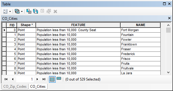 |
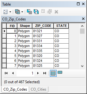
| In the CO_Zip_Code polygon layer (also, as noted by the Shape field) we note there is a field for the zip_code and a field for the state (which is Colorado, also noted by the name of the layer). | In the CO_Cities point A GIS vector data in any sort of digital science or art, is simply denoting a type of graphical representation using straight lines to construct the outlines of objects geometry type which is made up of just one vertex pl. vertices One of a set of ordered x,y coordinate pairs that defines the shape of a line or polygon feature. , marking a single XY location in any given geographic or projected coordinate system. layer (as noted in the Shape field) we note that the only fields in this layer is called "Feature" and has values referring to the population and a field for the Name of the city. |
 |
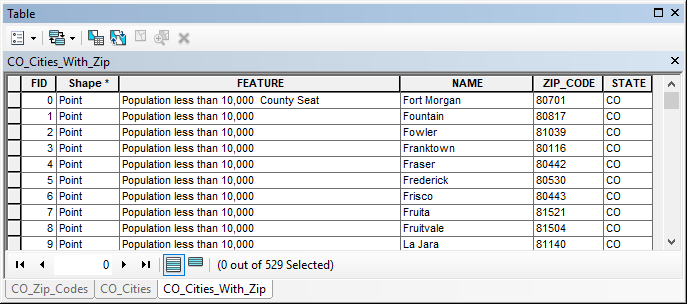 |
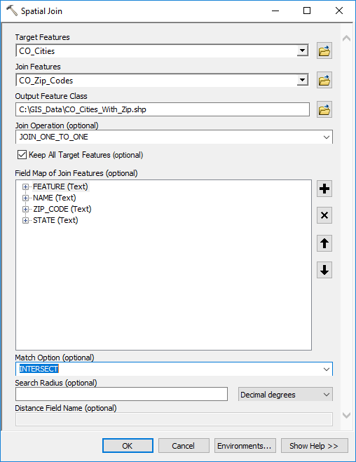
| The Spatial Join geoprocessing tool. The "joined to" layer (aka the Target Features) are the CO_Cities; the "joined from" layer (aka the Join Features) are the CO_Zip_Codes polygon layer. We notice the relationship type is one-to-one, meaning that each CO city has only one matching CO zip code and the Match Type (the two layers spatial relationship) is set to intersect, meaning that each city will gain the zip code of the polygon it falls inside. | The attribute table of the resulting CO_Cities_With_Zip layer. We note that attribute table contains all the fields from both layers and the resulting geometry type is equal to that of the "joined to" or Target Features. In the case of spatial joins, it may be necessary to spot check the accuracy of some of the features or look for any points that may have fallen exactly on the border of two of the polygons, as ArcMap may need some help deciding which polygon that point A GIS vector data in any sort of digital science or art, is simply denoting a type of graphical representation using straight lines to construct the outlines of objects geometry type which is made up of just one vertex pl. vertices One of a set of ordered x,y coordinate pairs that defines the shape of a line or polygon feature. , marking a single XY location in any given geographic or projected coordinate system. should have fallen in. |