Section Four - Meet ArcMap

In this section, we are going to take a look at ArcMap. Much like the last section, we are going to highlight some of the basic features; where to find them, what they do, etc. By the end of the semester, you shouldn't have to look most of these actions up, you should just have them down (but if you need to, this page is found here and when you click the ArcMap button in the top menu of the Wiki).

4.4.2: The Layout Of ArcMap

ArcMap, based on the definition of GIS, is a software to create, store, manage, analyze, and display data. While much of the storage and management is handled with ArcCatalog, there is some of that in ArcMap. ArcMap, however, is the portion of the software suite that was designed to create, analyze and display that data. We can use ArcMap to look at our data, explore our data, examine spatial relationships between our data, run geoprocessing tools and analyze the results, and create cartographic layouts to display the data to our customers (or instructor, in the case of this class).

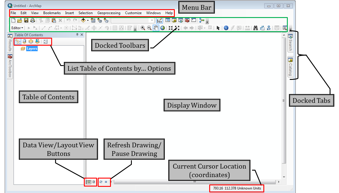
We see the basic layout is the same as ArcCatalog with a series of menus at the top above several toolbars of shortcut buttons, a thin Table of Contents which shows the layers participating in the ArcMap session, a large white space for interacting with the data, and some tabs along the right and left sides of the window hiding some additional toolboxes and windows.

Figure 4.5: ArcMaps's Basic Layout

4.4.3: Views and Areas of ArcMap

This first section will look at the major areas inside the ArcMap window where we list and interact with our data. Understanding the basic layout of ArcMap will help familiarize you with what to expect the first time you turn the software on instead of a surprise.

Data View vs Layout View

Since ArcMap is used to analyze and display our data, we have two distinct views in the software: data view and layout view. Data view is where we spent the majority of our time (compared to ArcCatalog and layout view), as the majority of our work is done creating and manipulating spatial data. Once we've taken the time to examine the data in great detail, both in the way the features, or the shapes representing real world objects, and the attributes in the attribute table, we switch over to layout view to complete the cartographic layout. Switching can be accomplished via the "View" menu at the top of the software window and a couple of shortcut buttons at the bottom of the display window, which we will look at next.

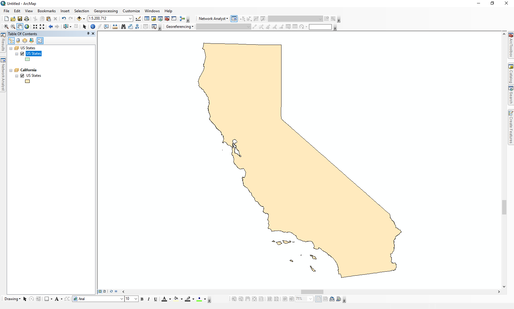
Figure 4.6: Data View vs Layout View in ArcMap
US States and California in Two Data Frames, Data View	US States and California in Two Data Frames, Layout View

Display Window and Data Frames

The Display Window is the portion of ArcMap where you interact with your data, showing us both data view and layout view. In data view, the layers draw, you can pan around, zoom in and out on, and interact with your data. In layout view, you can add map elements such as a north arrow, and a legend to create a final cartographic layout. This area is the main focus of ArcMap and the part you are going to spend the most time looking at. The Table of Contents list the data shown (by default) to the left of this area, the results of tools are loaded into this pane, and you create new data while looking at this area.

When you are looking at the Display Window in data view, you are looking at one Data Frame. A data frame is a collection of data layered to draw in a specified order in one geographic or projected coordinate system. While you can have more then one data frame in one MXD, ArcMap's data view will only show one at a time, or the active data frame, while layout view will show all of them at once in order to create final maps with several views, such as inset maps (maps which zooms in on a smaller area to show it in greater detail or shows the overall location of the data within some larger area of context) or different data for the same area, where overlapping that data would be impossible or confusing to the reader. Another use of additional data frames is the ability to eliminate white space when the portion of the map which matters covers a large area, such as details about the lower 48, Alaska, and Hawaii.

Figure 4.7: Data Frames in ArcMaps's Data View
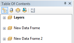	Data frames look like a stack of yellow squares, representing layers of data within the map. This yellow square is a repeating theme throughout ArcMap. In the next section, we will see how we add data to an MXD, where we will note the button icon is a yellow square with a plus sign. The first data frame will always be named "Layers" All other data frames will be named "New Data Frame", "New Data Frame 2", etc. The "active" data frame (the one displayed in Data View) will be listed in bold.

Data Frame Coordinate System

We learned all about coordinate systems in Chapter Two, noting that there are two major categories: geographic coordinate systems and projected coordinate systems. All spatial data is stored in a single coordinate system, either a geographic or a projected system. Knowing what coordinate systems a layer is stored in is very important, since it tells us how the data was created, what distortions may be present, and what units the displayed coordinates are in, since the measured units - angular or linear - are actually a measurement from the origin of the system in the X and Y directions to the feature being displayed. Longmont CO is found roughly at 40° N 105° W, meaning it is 40 degrees measurement of plane angle, representing 1⁄360 of a full rotation (circle). In full, a degree of arc or arc degree. Usually denoted by ° northwest of the origin of the latitude also known as 'parallels' the east-west portion of a geographic grid measured with angles between 0 and 90° and longitude geographic grid the result of using an established angular unit of measure to label the intersections of north-south and east-west lines on the surface of the Earth starting the labels at a principal meridian the north-south line from which the labeling begins.  East-west lines have a very obvious start point: the equator.  North-south lines must start somewhere, so when it is established for a particular geographic grid, it can be considered the principal meridian. , found under the "wing" of Africa.

We have the ability to change the stored coordinate system of a spatial layer via a tool called "Project", which looks at where the coordinates of features in one system correspond to the coordinates of another system, and reassigns those coordinates accordingly. For example, the latitude also known as 'parallels' the east-west portion of a geographic grid measured with angles between 0 and 90° and longitude coordinates of Longmont, more specifically 40° 10' 1.944" N 105° 6' 6.939" W, equate to the Universal Transverse Mercator (UTM) coordinates: Zone 13N, E: 491320.76 N: 4446320.79 (measured in meters from the origin of the 13N Zone). If we run a tool to convert the stored coordinate system for a US City Center point shapefile from the WGS84 Latitude and Longitude Geographic Coordinate System to the UTM Projected coordinate system, the tool will look at Longmont's latitude also known as 'parallels' the east-west portion of a geographic grid measured with angles between 0 and 90° and longitude in the input layer and find the UTM equivalent, overwriting the spatial data coordinates for the city in the output layer.

Figure 4.8: Changing the Display Coordinate System
Click to Hide/Show Animation
The display coordinate system can be changed without consequence to the stored coordinate system of the data listed in the Table of Contents. When the display coordinate system is changed, ArcMap projects the data on the fly, or shows what the data would look like if a tool such as Project was run.

ArcMap allows us to look at several spatial layers at one time in one data frame, regardless of what coordinate system the data is actually stored in, lining up the data the best it can for the user to interact with. We call this process projecting on the fly, meaning it is not creating a real change of the data, like would happen if we ran the Project tool), but instead displaying the hypothetical result as though the tool had run. We can change the display coordinate system of the data frame to our heart's content, and each time, ArcMap will project on the fly, redrawing each spatial layer in a display to match the selected data frame coordinate system.

How Do I Know a 'Real' Change is Happening with My Data?

This, and future chapters, will present options and actions and state they do not fundamentally change the data - meaning that nothing about the data will be permanent. ArcGIS is for displaying data, and can display data in several forms at once, without changing it. The best way to remember if you data is being fundamentally changed or simply changing how the data is being displayed is: Arc will ask you before changing data. For example, if you were presented with a confirmation box stating "Would you like to save your edits?", you most likely initiated the changes. When you run geoprocessing tools (Chapter Seven), the tool will offer a place to save the "output layer". This actually creates a new layer, complete with whatever changes were initiated - such as using the "Project" tool which produces a new spatial layer output stored in a different coordinate system than the input layer.

Current Cursor Location

Since the data frame is displayed in a single coordinate system, the display window can show you the coordinates of the cursor at any given time. These current cursor coordinates are shown at the bottom of the display window in the coordinate system of the data frame regardless of the coordinate system of each layer participating in the ArcMap session, and as you move your cursor around the window, the coordinates change. These current cursor coordinates are useful in getting a rough idea of where you are looking in the world while you are working within ArcMap. For example, if you add some data that you know is in Central Colorado and the current cursor coordinates are displaying values of 85° N, 115° E when you move your cursor over the data, you can quickly get a pretty good idea that something is wrong with the data.

Figure 4.9: Current Cursor Coordinates in Action
Click to Hide/Show Animation
Both ArcMap and ArcCatalog (Preview Window) show the current cursor coordinates at the bottom of the window. Notice in the animation that the coordinates scroll while the cursor is moving and pause when the cursor pauses.

When you switch over to layout view in ArcMap in order to start creating your cartographic product, a second set of cursor coordinates pop up, showing you map coordinates, a positive set of coordinates referring to where your cursor is on the printed page versus where the data is in the real world. The coordinates are based on the same principles of the Cartesian Coordinate System, where the is an origin at the lower left corner of the page and positive values moving along the X and Y axis of the page itself. The concept is exactly the same a projected coordinate system, where there is some origin somewhere in the world, and to locate places on the Earth's surface, we move away from the origin until we arrive, measuring the distance in linear units.

Figure 4.10: Map Coordinates Displayed in Inches
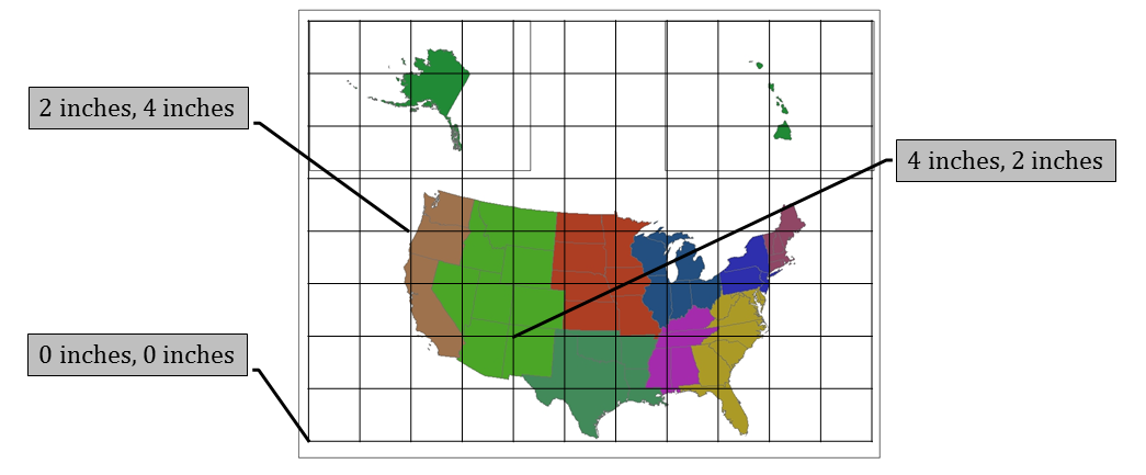To locate map elements (legend, title, north arrow, etc) for printing neatly and evenly spaced, ArcMap's Layout View uses map coordinates. Also based on the Cartesian Coordinate System, map coordinates are positive numbers starting at a 0,0 origin found at the lower left corner of the page.

Table of Contents

In ArcMap, the Table of Contents is the window where all of your spatial layers and data tables are displayed. Some of them might be visible, some may not, some might have special styling, others may be just tables. Regardless of how the data is displayed in your map, all of the active layers are listed in the Table of Contents. From here, you can move the data to draw in a different order, see where data is stored on your computer, and examine how different layers are displayed. You can add data to the map, remove data from the map, make changes to the display of the active layers, and access information about each layer.

As ArcMap is the software in the suite used to interact with our data and create cartographic layouts, we have the ability to make display changes, such as the color of the features when they draw on the map, whether or not we can see feature labels like state names when a US states layer is active, or which layer draws on top of the next. These display changes are not fundamental changes to the data, as it really makes no difference if that US States layer is displayed in light green every single time it's added to an ArcMap project. The five to eight little files each shapefile is made up of dictate things like where each feature lives in the world, what coordinate systems the data is stored in, the coordinates of those features, and the attributes about the features - the non-spatial values which we can attribute to each feature. Not a single one of them dictate what color to fill in each state with, what color the outline line should be, or if the labels are visible or not (labels, however, are attributes, such as the name of each state). Those are all cartographic decisions made by a GIS technician each time they use the US States layer. In one project, the layer might be used for analysis and needs to be featured at the front of the map, and in another map, the states might just be used for context, or features which help visually locate other features in the world.

Since ArcMap can show us lots of information about our data - what it looks like and what order to draw it in, where it's stored on the computer, what layers are visible or hidden at any given time, or if selections have been made in the attribute table (Chapter Five), and ESRI (the company who makes ArcGIS) has no idea what you need to look at when, the Table of Contents offers us four different ways to list our data. We call these the List by... Options, and in this section, we will quickly look over three of the four just to get an understanding that ArcMap can show us data in different ways, not necessarily to memorize each view right now.

List by Drawing Order
This is the default view which ArcMap loads into. With this view you can: Turn layers on and off by checking and unchecking the box to the left of the layers name Re-order layers by dragging the name to another place in the list. Feature classes draw in layers, thus the top of the list will be the 'top of the pile'. If you can't see a layer and it is turned on, it is likely covered by another layer. Try dragging it higher in the list to view it. You can see where the layer is going by the dark black line which appears between layer names as you move your mouse around Sometimes its hard to drop a layer at the top of the list for simple reasons of it's not cooperating with you. Try dropping it in the second place and dragging the top layer below it. Change layer symbology Access the Layers Option menu for each layer	Click to Hide/Show Animation
List by Source
List by source shows where each layer is stored. It organizes the data into groups based upon where the data is saved. For example, all the feature classes found in the Example.gdb geodatabase are in one group followed by all the shapefiles stored in the Example folder. Two major differences between List by Drawing Order and List by Source are: You cannot drag the layers to reorder them. In fact, you can't reorder them at all. You can see where the layers are stored/saved without accessing the properties of each individual layer
List by Visibility
List by visibility groups all of your layers based into two groups: Visible and Not Visible. Visible layers are set to draw and be shown in the Display window while Not Visible layers are still participating in your map, but are prevented from drawing or displaying. If you are working with a map with just few layers, like a GIS 101 lab, this option is no different then simply checking and unchecking the boxes in List by Drawing Order, however, when your projects grow in size and the Table of Contents is full of layers, especially if you group your layers, you may need to see just what layers are set to be visible and which ones are not. You can think about List by Visibility like grouping apps on your phone. You see the group heading and know inside the Fitness group are all of your running apps, but it isn't until you open the group that you can see exactly which apps are participating in that group.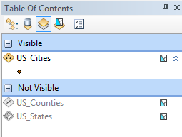

Turning Layers On and Off and Collapsing and Expanding Layers

We've looked at the Display Window and the Table of Contents within ArcMap, stating that the layers participating in the current ArcMap session are listed out in the Table of Contents can be set to draw or not draw in the Display Window and can be reordered so certain layers draw on top of other layers. From this, we can derive the fact that not every spatial layer on the computer is visible at once in ArcMap and that we would need to intentionally add the data to the MXD. While we will look at all the ways we can add data to an ArcMap session, the how isn't the most important thing right now, but the fact that we can and from there, we can control which layers are visible and which are not.

Similar to adding an image to a Word document or your social media page, adding data to ArcMap involves opening a dialog box, looking in folders - and in the case of spatial data, geodatabases - until you find the layer you wish to add. Once you've found it, it's a matter of clicking on it's name and confirming your selection with some sort of "OK" or "Add" button. When you add a layer to ArcMap it automatically draws it in the Display Window and places itself at the top of the Table of Contents. The choice for it to draw or not is controlled by checking the corresponding box in the Table of Contents.

In addition to automatically drawing each layer when it is added to a map session, the layer is added expanded, where a color patch showing the color, line pattern, or point graphic the layer is being represented as is listed below each layer name. For polygons, the patch is a rectangle, for polylines, it is a single straight line, and for points, it is the same graphic as the points are being displayed in the map. These examples allow for you to look at the Table of Contents and locate the color or symbol of a particular layer in the map, similar to using a legend in a completed cartographic product, as well as have quick access to the dialog boxes which change said color or symbol. Since the layer is expanded when it's added, you have to option to collapse it and hide the patch from view, regardless if the layer is drawing in the display window or not.

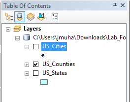
Figure 4.11: Collapsing/Expanding and Turning On/Turning Off Layers in the Table of Contents within ArcMap
The check box for the states layer is checked, which means it will draw in the display window.	In this screenshot, the states layer is expanded, showing the blue patch representing the color the polygon will fill in with. The rivers layer is collapsed, meaning whatever color the line draws in is currently hidden from view.

4.6.4: Menus And Toolbars

ArcGIS has a series of menus and toolbars which are most often found at the top of the window. Menus have tons of functionality, and many sub-menus with even more options. Toolbars are series of buttons which are either shortcut buttons for actions found in menus or control actions for a process within the software, such as all the buttons we would use to draw new features in our map (Chapter Six). Again, the list here is not for you to memorize, as that will simply come in time, but for you to see that there is quite a bit of functionality in ArcMap, and the software programmers do their best to organize those functions in a logical manner. The toolbars displayed are just three of (lots), two are examples of shortcut buttons for the Menus and one is an example of buttons for specific functionality, in this case, for changing and creating new features.

Menu Name	Highlights
File	New and save MXD, print, and important to turning in your labs, the Export Map option to save your MXD as a PDF
Edit	For now, the most important thing in Edit is "Undo"
View	Switch between Data View and Layout View and the option pause drawing if it's drawing very slow
Bookmarks	Creates bookmarks in your MXD to save the current view and return to it later
Insert	Insert a new data frame; map elements (title, legend, scale bar) when working in Layout View
Selection	How to highlight data you'd like to interact with.
Geoprocessing	The "Top Six" tools used to save spatial problems. Covered in Chapter Seven. The "Results" window which shows the inputs and messages from all the geoprocessing tools run in an ArcMap Session.
Customize	A list of toolbars available; the enable extension options (covered on the next page)
Windows	Different views to interact with your data better; where to get your Table of Contents back when you lose it
Help	Launches your best friend in the ArcGIS world, the help menu
Standard Toolbar	The Standard toolbar has buttons which control the MXD (save, open, etc), add data to the MXD, and open additional windows (described below)
Tools Toolbar	The Tools toolbar has functions used to navigate the map (pan, zoom, etc) and explore the data in spatial way (measuring features, finding a XY location, etc)
Editor Toolbar	The Editor toolbar contains a series of buttons used to draw new vector features (you create the dot to dot with your mouse by placing each vertex where it belongs in the world) and edit existing ones (change how the polygon or polyline are drawn, moving a point from one place to another)

4.4.5: Additional Windows in ArcMap

The Table of Contents is not the only window available in ArcMap, even though it is the most common. Other windows allow you to find tools to analyze your data, search for tools or spatial data on your computer, and bring in the Catalog Tree without having to open ArcCatalog in a separate window. These windows add ease an functionality to the way that ArcMap works. Just to sound like a broken record, this section is not here for you to memorize the things ArcMap does, but see that we interact with the software and spatial data in several ways beyond just adding data to the Table of Contents and examining it in the display window, hoping it will do a trick or provide us with an ice cream cone on a hot day.

ArcCatalog Window

The ArcCatalog Window is basically like having the Catalog Tree tacked to the side of ArcMap. Anything you can accomplish in the Catalog Tree, such as creating, renaming, moving, and deleting folders, shapefiles, geodatabases, and feature classes, can be done in the ArcCatalog Window. The benefit to having a 'peek' at the Catalog Tree is simply not having to launch ArcCatalog, as well as the two instances stay in sync (as you move through this class, you will notice that ArcMap and ArcCatalog work on a cache, meaning it doesn't instantaneously update any changes you've made to data from ArcCatalog to ArcGIS without forcing it to refresh.. We will get to that.)

Search Window

The Search Window can search for all thing GIS. You can find layers, MXDs, images, and what we will be using it for, tools in the ArcToolbox.

ArcToolbox

The ArcToolbox Window houses all of the geospatial tools available in ArcGIS. The tools are grouped by like features, such as all the tools we use to compare how layers relate to each other spatially. In that group we might find tools that calculate what percentage of one layer is intersecting another, or a tool that will remove all parts of a layer that do not intersect with another.

In this class, you will be guided to particular toolboxes to perform certain tasks. However, knowing they are grouped together might help you find a tool for your final project or solve a problem you didn't even know you had! (Honestly, I've found more tools by looking for other tools then knowing the tool existed in the first place.)

Docking Windows

Along with the Table of Contents there are other windows that can be docked along the sides of the ArcMap window to access data, tools, or ArcCatalog without launching ArcCatalog. The four most common tabs docked are: ArcCatalog, the Search Window, ArcToolbox, and the Results Window.

Figure 4.12: Windows in ArcMap Can Be Free Floating or Attached (Docked) to the Side of the Display Window
Click to Hide/Show Animation
Click to open a tab. Drag to a blue arrow to dock. Push pin lying on its side = Auto Hide. Push pin facing down = Stays put/ready to be dragged to a new location. X = close the window completely (not the same as auto hide)